The Latest in

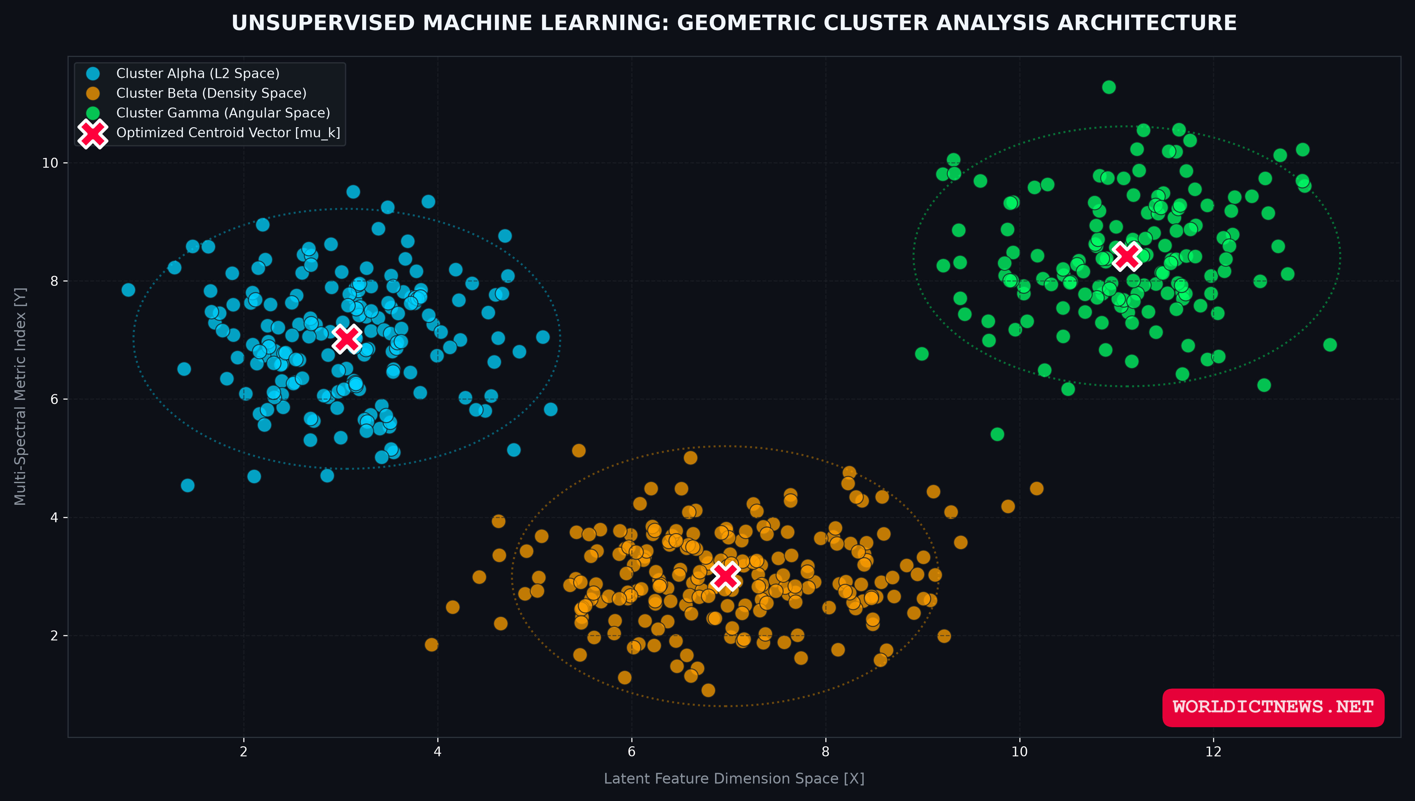
The Architecture of Cluster Analysis: Mathematical Frameworks, Algorithmic Blueprints, and Production Python Architectures. In the era of big data, organizations ingest massive volumes of unlabelled, multi-dimensional information every second. Whether processing high-frequency e-commerce transaction logs, streaming multi-spectral satellite telemetry, or managing clinical patient biometric profiles, data scientists face a common hurdle: finding meaningful, hidden structures in data without pre-existing training labels.Traditional machine learning relies heavily on supervised paradigms like classification and regression. However, supervised models are fundamentally helpless when a business does not possess historical target outcomes or categories. To uncover the organic taxonomies, underlying customer personas, or anomaly vectors buried within unlabelled datasets, we must deploy Cluster Analysis.Cluster analysis (or clustering) is the unsupervised task of grouping a set of data objects into distinct partitions. The structural goal is straightforward: maximize intra-cluster similarity (objects inside the same cluster should be as close to one another as possible) while maximizing inter-cluster disparity (separate clusters should be as distinct and distant from one another as possible).This comprehensive masterclass breaks down the foundational math of distance spaces, analyzes three major algorithmic paradigms (Centroid-based, Density-based, and Hierarchical), evaluates clustering quality using rigorous verification metrics, and provides a production-grade Python workflow with real-world business case studies.1. The Mathematical Core: Proximity Measures and Distance SpacesAt the center of every clustering algorithm sits a proximity metric. Because unsupervised models lack historical outcome labels to judge correctness, they rely on geometric distance calculations to define what makes two observations "similar."The selection of a distance space determines the geometric shape of the resulting clusters. If you change the metric, you alter how the algorithm maps boundaries across the feature grid. ┌──────────────────────────────┐ │ Distance Spaces │ └──────────────┬───────────────┘ │ ┌───────────────────────┼───────────────────────┐ ▼ ▼ ▼ [ Euclidean ] [ Manhattan ] [ Cosine Space ] Straight-Line (L2) Grid-Based (L1) Directional Angle Euclidean Distance (L2 Norm)The most common geometric metric used in data science is Euclidean Distance. It calculates the straight-line distance between two coordinates in a multi-dimensional Cartesian space.Plain-Text Formula: For two n-dimensional observations, P = (p1, p2, ... pn) and Q = (q1, q2, ... qn), the Euclidean distance is defined as:Distance(P, Q) = sqrt( sum( (pi - qi)^2 ) )Operational Caveat: Euclidean space assumes all features are continuous, normally distributed, and scaled equally. If one feature represents annual revenue in millions and another represents customer age in years, the revenue variable will completely overwhelm the calculation. Therefore, standardizing features via Z-score normalization or Min-Max scaling is a mandatory pre-requisite before applying Euclidean-based models.Manhattan Distance (L1 Norm / Taxicab Geometry)Instead of cutting diagonally across coordinates, Manhattan Distance measures the path along axes at right angles.Plain-Text Formula:Distance(P, Q) = sum( abs( pi - qi ) )Operational Fit: Manhattan distance is highly robust when analyzing datasets with high dimensionality. As the number of dimensions scales upward, Euclidean distances tend to become uniform (a phenomenon known as the curse of dimensionality). The L1 norm helps preserve contrast between data points in dense feature environments.Cosine Similarity & DistanceWhen the absolute magnitude of features matters less than the relative direction or orientation of the data vectors, we shift to Cosine Space. This is standard in text mining, natural language processing (NLP), and user recommendation systems.Plain-Text Formula: It calculates the cosine of the angle theta between two multi-dimensional vectors:Similarity(P, Q) = cos(theta) = (P dot Q) / (norm(P) * norm(Q))Cosine Distance = 1 - Similarity(P, Q)Operational Fit: If you are clustering documents based on word frequencies, a short 100-word article and a massive 10,000-word essay might cover the exact same topic. Euclidean distance will mark them as incredibly far apart due to total word counts. Cosine distance looks strictly at the vector angle, correctly clustering them together based on proportional keyword alignment.2. Core Algorithmic FrameworksNo single clustering algorithm fits every dataset. Data structures vary: some consist of neat, spherical groups, while others form winding, intertwined density paths. Data scientists choose models from three major structural families.Family A: Centroid-Based Models (K-Means)K-Means is the workhorse of unsupervised learning. It aims to partition N observations into K distinct clusters, where each observation belongs to the cluster with the nearest mean (centroid). [ Initial Random Centroids ] ──► [ Assign Points to Nearest Mean ] ──┐ ▲ │ └─────────────── [ Recalculate Centroid Means ] ───────┘ The model iteratively optimizes the Within-Cluster Sum of Squares (WCSS), also known as Inertia:WCSS = sum_k( sum_xi_in_Ck( norm( xi - mu_k )^2 ) )Where Ck is the set of points in cluster k, and mu_k is the calculated mean centroid of that cluster.The Operational Lifecycle of K-Means:Initialization: The user specifies the exact number of clusters (K). The algorithm places K random starting centroids across the feature grid (often using the advanced k-means++ initialization routine to spread them out efficiently).Assignment Step: Every observation in the dataset is assigned to its closest starting centroid based on Euclidean distance.Update Step: The algorithm calculates the geometric mean of all coordinates assigned to each cluster, moving the centroids to these new center points.Convergence: The Assignment and Update phases loop continuously until the centroids stop shifting or the maximum iteration threshold is hit.Structural Weakness: K-Means assumes clusters are spherical, roughly equal in size, and have similar density spreads. It fails completely when confronted with complex geometric patterns, elongated configurations, or heavy background noise.Family B: Density-Based Models (DBSCAN)DBSCAN (Density-Based Spatial Clustering of Applications with Noise) approaches data by grouping points based on spatial concentration rather than center points.Unlike K-Means, DBSCAN does not force you to guess the number of clusters in advance. It identifies clusters of arbitrary shapes and automatically flags isolated data points as background noise.Core Structural Parameters:Epsilon (Eps): The maximum radius distance to search for neighboring points around a coordinate.MinSamples: The minimum number of points required within the Epsilon radius to declare that area a dense region.The Classification of Data Points:Core Points: Any coordinate that contains at least the MinSamples count inside its Epsilon neighborhood.Border Points: Points that do not have enough neighbors to be core points, but fall inside the Epsilon radius of a valid Core Point.Noise Points (Outliers): Any observation that is neither a Core Point nor a Border Point. These are ignored by clusters, making DBSCAN highly resilient to anomalies. ( Core Point ) ──► [ High neighbor density within Epsilon ] ( Border Point ) ──► [ Low neighbor density, but touches a Core Point ] [ Noise Point ] ──► [ Isolated outlier; excluded from all clusters ] Structural Weakness: DBSCAN struggles when analyzing datasets with highly variable densities. If one cluster is tightly packed and another is loosely spread, a single Epsilon value cannot capture both boundaries cleanly.Family C: Hierarchical Models (Agglomerative)Agglomerative Hierarchical Clustering builds a tree of clusters using a bottom-up methodology.The Assembly Pipeline:Every observation starts as its own individual single-point cluster (N items = N clusters).The algorithm calculates the distance between all clusters and merges the two closest ones into a joint group.The merging loops continuously until all observations are unified into a single root cluster.Linkage Matrix Criteria:To determine the distance between clusters containing multiple points, developers choose specific linkage parameters:Ward Linkage: Minimizes the total variance increment within clusters during merges. This yields highly spherical, balanced clusters.Complete Linkage: Computes the distance between the two furthest points across clusters.Single Linkage: Computes the distance between the two closest points across clusters. This is prone to chaining effects, where trailing noise points accidentally bridge distinct clusters together.The entire hierarchical structural tree is visualized using a graphic called a Dendrogram. This allows practitioners to visually cut across branches to choose the optimal number of clusters after the processing phase completes.3. High-Value Business Case Study: Customer Segmentation Workflow in Python💼 Business ContextAn international e-commerce platform wants to optimize its seasonal marketing campaigns. Rather than blasting millions of generic promotional emails to their entire user base, they want to isolate distinct customer purchasing personas based on transaction values, website interaction metrics, and loyalty patterns.🎯 ObjectiveSimulate a production-level dataset of 500 customers, execute data preprocessing, determine the optimal cluster configuration using diagnostic indices, deploy an optimized K-Means engine, and output high-resolution visualization profiles.🛠️ Production Verification CommandTo execute this analytical workflow natively inside Visual Studio Code, ensure your system terminal has the required data science library suite installed:bashpip install numpy pandas matplotlib seaborn scikit-learn Use code with caution.Python Blueprint Implementation (customer_segmentation.py)pythonimport numpy as np import pandas as pd import matplotlib.pyplot as plt import seaborn as sns from sklearn.preprocessing import StandardScaler from sklearn.cluster import KMeans from sklearn.metrics import silhouette_score, calinski_harabasz_score # ========================================== # 1. GENERATE SYNTHETIC CUSTOMER TRANS_LOGS # ========================================== np.random.seed(42) # Generate three distinct target populations (Personas) # Group 1: High Spending, Low Engagement (VIP Bargainers) g1_spend = np.random.normal(loc=120, scale=15, size=150) g1_engage = np.random.normal(loc=30, scale=5, size=150) # Group 2: Low Spending, High Engagement (Loyal Browsers) g2_spend = np.random.normal(loc=40, scale=10, size=200) g2_engage = np.random.normal(loc=85, scale=8, size=200) # Group 3: High Spending, High Engagement (Core Brand Champions) g3_spend = np.random.normal(loc=200, scale=25, size=150) g3_engage = np.random.normal(loc=75, scale=10, size=150) # Unified Data Frames Assembly df_spend = np.concatenate([g1_spend, g2_spend, g3_spend]) df_engage = np.concatenate([g1_engage, g2_engage, g3_engage]) df_customers = pd.DataFrame({ 'Annual_Spend_USD': df_spend, 'Engagement_Score': df_engage }) print("--- RAW CUSTOMER TRANSACTION LOG METRICS ---") print(df_customers.head()) print(f"Total Customer Datasets: {df_customers.shape} Rows\n") # ========================================== # 2. DATA PREPROCESSING & STANDARDIZATION # ========================================== # Standardize features to have a mean of 0 and variance of 1 scaler = StandardScaler() scaled_features = scaler.fit_transform(df_customers) # ========================================== # 3. DIAGNOSTIC SCANS: TARGET SELECTION # ========================================== wcss_inertia = [] silhouette_coefficients = [] k_range = range(2, 11) for k in k_range: kmeans_eval = KMeans(n_clusters=k, init='k-means++', random_state=42, n_init=10) kmeans_eval.fit(scaled_features) wcss_inertia.append(kmeans_eval.inertia_) silhouette_coefficients.append(silhouette_score(scaled_features, kmeans_eval.labels_)) # Plot Diagnostic Curves (Elbow and Silhouette) fig, (ax1, ax2) = plt.subplots(1, 2, figsize=(16, 5)) # Elbow Method Plot ax1.plot(k_range, wcss_inertia, marker='o', color='#1A365D', linewidth=2) ax1.set_title('Elbow Validation Diagnostic: Minimizing WCSS', fontsize=11, fontweight='bold', color='#1A365D') ax1.set_xlabel('Cluster Count (K)') ax1.set_ylabel('Within-Cluster Sum of Squares (Inertia)') ax1.grid(True, linestyle='--', alpha=0.5) # Silhouette Analysis Plot ax2.plot(k_range, silhouette_coefficients, marker='s', color='#2B6CB0', linewidth=2) ax2.set_title('Silhouette Framework Scan: Maximizing Separation Coeff', fontsize=11, fontweight='bold', color='#2C5282') ax2.set_xlabel('Cluster Count (K)') ax2.set_ylabel('Average Silhouette Coefficient') ax2.grid(True, linestyle='--', alpha=0.5) plt.tight_layout() plt.savefig("clustering_diagnostics.png", dpi=300) print("DIAGNOSTIC VISUALIZATION LOGGED: 'clustering_diagnostics.png' saved to disk.") # ========================================== # 4. OPTIMIZED ENGINE DEPLOYMENT (K=3 chosen) # ========================================== optimal_k = 3 final_engine = KMeans(n_clusters=optimal_k, init='k-means++', random_state=42, n_init=10) cluster_assignments = final_engine.fit_transform(scaled_features) df_customers['Cluster_ID'] = final_engine.labels_ # ========================================== # 5. METRIC QUANTIFICATION MATRIX # ========================================== sil_avg = silhouette_score(scaled_features, final_engine.labels_) ch_score = calinski_harabasz_score(scaled_features, final_engine.labels_) print("\n=== SYSTEM PERFORMANCE EVALUATION METRICS ===") print(f"Final Configured Clusters (K): {optimal_k}") print(f"Average Silhouette Score: {sil_avg:.4f}") print(f"Calinski-Harabasz Variance Score: {ch_score:.2f}\n") # ========================================== # 6. PRODUCTION SUMMARY CLUSTER SEGMENTS # ========================================== cluster_profile_summary = df_customers.groupby('Cluster_ID').mean() print("=== CLUSTER PROFILED MEAN SEGMENTATION SUMMARIES ===") print(cluster_profile_summary) # ========================================== # 7. HIGH-RESOLUTION EXPEDITION GRAPH # ========================================== plt.figure(figsize=(12, 8)) sns.scatterplot( data=df_customers, x='Annual_Spend_USD', y='Engagement_Score', hue='Cluster_ID', palette=['#1A365D', '#DD6B20', '#2F855A'], s=100, alpha=0.8, edgecolor='w' ) # Convert Centroids back to original unscaled feature parameters for plotting unscaled_centroids = scaler.inverse_transform(final_engine.cluster_centers_) plt.scatter( unscaled_centroids[:, 0], unscaled_centroids[:, 1], s=350, color='red', marker='X', edgecolor='black', linewidth=2, label='Optimized Cluster Centroids' ) plt.title('Systems Analytics Workspace: Corporate Customer Segmentation Engine', fontsize=13, fontweight='bold', color='#1A365D') plt.xlabel('Annual Customer Spend Architecture (USD / Year)') plt.ylabel('Digital Interface Engagement Index Score (0 - 100)') plt.grid(True, linestyle=':', alpha=0.6) plt.legend(loc='upper right') plt.savefig("customer_segmentation_output.png", dpi=300) print("PRODUCTION METRIC MAP EXPORT SUCCESS: 'customer_segmentation_output.png' saved.") plt.show() Use code with caution.4. Mathematical Validation Frameworks: Interpreting the ScoresBecause cluster analysis does not check its outputs against predefined ground-truth labels, models can easily group random noise into arbitrary clusters. To ensure our generated clusters represent real physical boundaries rather than statistical alignment artifacts, we rely on two key validation frameworks:1. The Silhouette CoefficientThe Silhouette Score measures how clean the geometric separation between clusters is. For an individual observation i, its silhouette coefficient s(i) is defined as:s(i) = ( b(i) - a(i) ) / max( a(i), b(i) )Where:a(i) is the mean intra-cluster distance between point i and all other coordinates in the same cluster. It maps compactness.b(i) is the mean nearest-cluster distance between point i and all points in the closest neighboring cluster. It maps separation.Interpretation Matrix:Near +1.0 Score: Points are located far away from parallel clusters, indicating a clean, highly resilient structural partition.Near 0.0 Score: The coordinate sits directly on the boundary line between two overlapping clusters, signaling high system ambiguity.Negative Score: The observation has been grouped into the wrong cluster entirely.2. The Calinski-Harabasz Index (Variance Ratio Criterion)The Calinski-Harabasz score computes the ratio of the sum of between-clusters variance to the within-cluster variance.CH Score = ( SSB / SSW ) * ( (N - K) / (K - 1) )Where SSB is the variance between different clusters, SSW is the variance inside individual clusters, N is the total number of observations, and K is the number of clusters.The Logic: A higher Calinski-Harabasz score indicates that the clusters are both tightly packed internally and spaced widely apart externally, making it an excellent diagnostic metric for choosing the optimal cluster count.5. Comparative Diagnostics Summary MatrixTo choose the optimal model layout across diverse feature environments, reference this baseline algorithm selection guide:Clustering AlgorithmTuning ParametersCluster Geometry CapOutlier Processing StrategyComputational ComplexityRecommended Domain FitK-Means EngineNumber of clusters (K)Spherical, convex groupings only.Forces outliers into centroids, distorting center means.Linear: O(N K I) -- Very fast on massive datasets.Rapid, high-volume consumer persona indexing.DBSCAN PipelineEpsilon (Eps), Minimum Samples count.Arbitrary shapes, loops, and winding density paths.Automatically filters noise points as non-classified anomalies.Quadratic: O(N^2) -- Slows down significantly on giant datasets.Geospatial geo-fencing, telemetry arrays, anomaly detection.Agglomerative MatrixLinkage criteria choice, Cut-off threshold.Dependent on linkage; single can chain, Ward builds spheres.Unifies outliers slowly into branches at high levels.Cubic: O(N^3) -- Inefficient for ultra-high-volume production tables.Small to medium biological taxonomies, genetic mappings.6. Operational Best Practices for Production DeploymentAlways Apply Feature Scaling: If your inputs use mismatched dimensions (e.g., matching a binary 0/1 gender flag against a $100,000 income column), distance-based models will focus entirely on the larger metric range. Apply Z-score standardization (StandardScaler) to give all features an equal footing.Mind the Curse of Dimensionality: As you add more variables to a dataset, the geometric volume of the space expands rapidly. This causes distances between points to become uniformly wide, making Euclidean metrics less effective. Use dimensionality reduction techniques like PCA (Principal Component Analysis) or t-SNE to compress your features down to core components before running your clustering models.Avoid Over-interpreting Inertia Curves: When running the K-Means Elbow method, the WCSS line will drop naturally every time you increase the cluster count (K), hitting zero when K equals the number of data points. Look for a clear, sharp bend in the curve where adding more clusters yields diminishing returns, and verify this point against your average Silhouette score.Establish Baseline Reproducibility: Because algorithms like K-Means pick random initial coordinates for their starting centroids, running the same script twice can yield slightly different results. Always fix your execution pipeline by setting a constant seed parameter (e.g., random_state=42) to guarantee your results are reproducible across production environments.

On September 22, 2026, U.S. President Donald Trump addressed the 81st United Nations General Assembly (UNGA) in New York, sparking global debate by re-branding Artificial Intelligence as "Super Intelligence" (SI). This rhetorical shift marks a definitive moment in technological geopolitics, directly challenging the United Nations’ efforts to build international regulatory frameworks.Redefining the Future: President Trump’s "Super Intelligence" Doctrine at the UNGAThe Rhetorical Shift: Why "Artificial" Fails, and "Super" WinsDuring his address to the United Nations General Assembly, President Trump explicitly took aim at the standard terminology used by global tech firms, researchers, and policymakers: "Artificial Intelligence". To a crowded assembly room of global leaders, he argued that the word "artificial" heavily undersells the capabilities and massive socio-economic scale of the technology.Trump argued that "artificial" makes intelligence sound fake, declaring that official documents would transition to the term Super Intelligence (SI). This rebranding treats the technology as a dominant expansion of cognitive power rather than a synthetic imitation. Following public name-testing that discarded alternatives like "Supreme Intelligence," SI was adopted as the formal U.S. government standard.Direct Rejection of Global AI Frameworks and Economic GrowthTrump used the UNGA podium to explicitly reject coordinated global regulatory schemes or limits on high-level models, maintaining that U.S. agencies can manage domestic issues without foreign oversight. Dismissing existential safety concerns as an innovation-stifling "hoax", the administration prioritized economic maximalism, with Trump asserting that SI will be "bigger than the Industrial Revolution" and drive breakthroughs across finance, automation, and infrastructure.Geopolitical Stance and Global FalloutDriven by a zero-sum race against China where America currently leads by a wide margin, the administration's stance avoids bureaucratic slowdowns that could erode U.S. tech supremacy. This unilateral pivot has introduced diplomatic friction with European allies favoring strict governance, created a fractured compliance landscape for multinational tech firms, and fundamentally altered the global terminology and terms of engagement surrounding technological primacy.

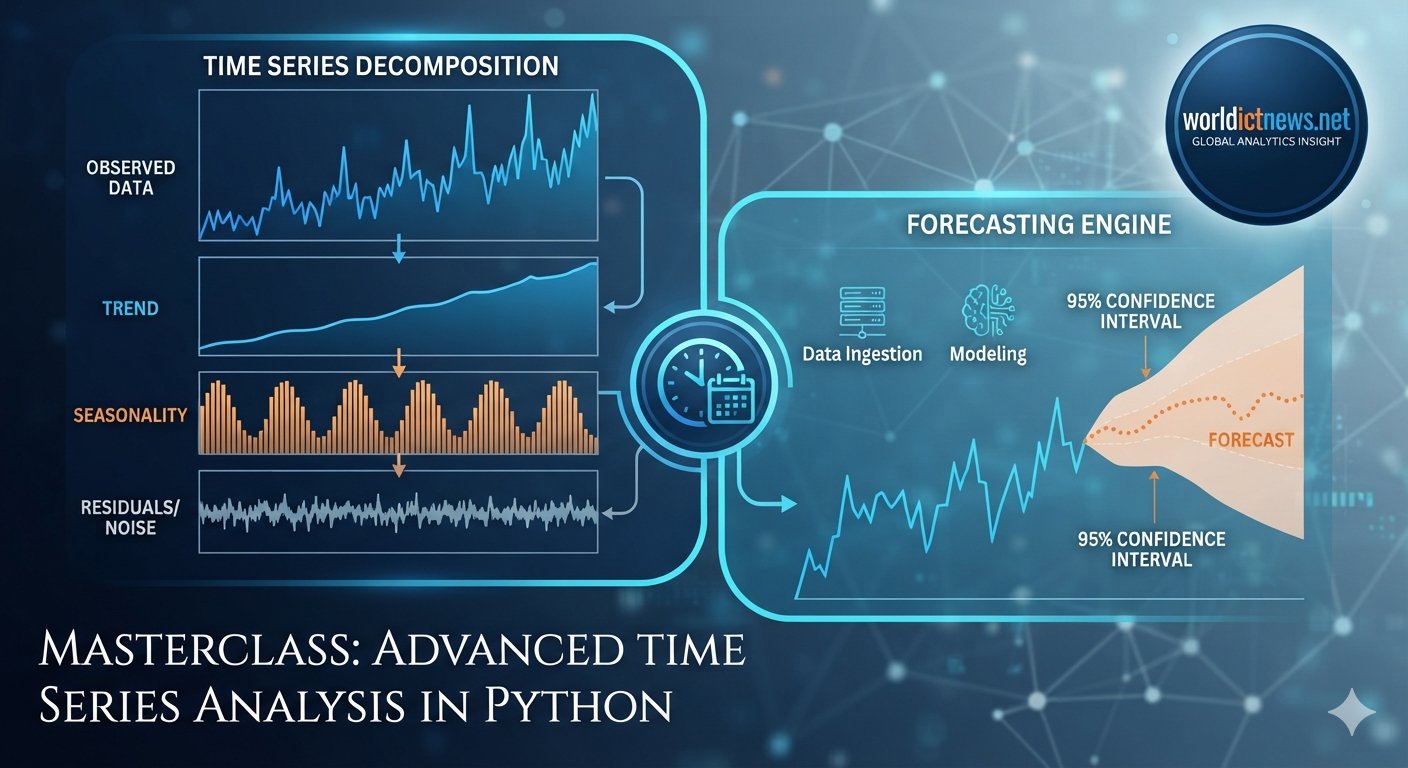
Masterclass: Advanced Time Series Analysis in Python. In data science, we frequently deal with cross-sectional data—snapshots of multiple entities at a single point in time, such as customer profiles, hospital patient metrics, or house prices across a city. However, in the real world, data rarely stands still. The most valuable business assets change over time: stock prices tick upward second by second, e-commerce servers log thousands of visitor clicks every minute, and cellular network towers experience traffic surges depending on the hour of the day.To analyze, model, and predict these dynamic systems, we must turn to Time Series Analysis (TSA).A time series is a sequence of data points recorded at consistent, successive intervals over time. Unlike standard statistical data where observations are assumed to be independent, time series data possesses an inherent chronological order. What happened yesterday directly influences what happens today, and what happens today heavily impacts what will happen tomorrow.This comprehensive guide unpacks the foundational concepts of Time Series Analysis, introduces the core statistical properties required to model temporal systems, examines structural decompositions, and provides deep, real-world examples equipped with production-ready Python implementations.1. Core Structural Properties of Time Series DataBefore applying forecasting models, we must dissect the structural DNA of a time series. A typical time series can be broken down into four distinct, overlapping structural elements:Trend: The long-term direction of the data over a prolonged period. Trends can be upward (e.g., global carbon emissions over decades), downward (e.g., desktop computer sales over the last ten years), or stationary/flat.Seasonality: Predictable, repeating fluctuations that occur within fixed, specific calendar periods. For example, retail sales spiking every December due to holiday shopping, or residential electricity consumption surging every afternoon during peak summer heat waves.Cyclic Patterns: Long-term oscillations that rise and fall over unpredictable, variable intervals. These are typically driven by macro-economic factors or business cycles (e.g., economic recessions occurring every 7 to 11 years). Unlike seasonality, cyclic patterns do not have a fixed, repeating calendar frequency.Irregular/Residual Component: Random, unpredictable noise or statistical variations. This represents the white noise left behind after the trend, seasonality, and cyclic forces are completely extracted. These are caused by sudden, exogenous shocks like geopolitical events, extreme weather mutations, or black swan market disruptions. ┌──────────────────────────────────────────────────┐ │ Observed Data │ └────────────────────────┬─────────────────────────┘ │ ┌─────────────────────────┼─────────────────────────┐ ▼ ▼ ▼ [ Trend ] [ Seasonality ] [ Residuals ] Long-Term Direction Calendar-Fixed Patterns Random White Noise The Concept of StationarityThe single most critical statistical constraint in traditional time series forecasting is Stationarity.A time series is considered strictly stationary if its statistical properties—specifically its mean, variance, and autocorrelation structure—remain completely constant over time.Why it matters: Most classical statistical forecasting architectures (such as ARIMA) operate under the assumption that the underlying data distribution is stable. If a time series has a shifting mean (an upward trend) or an expanding variance (volatility that grows over time), mathematical models cannot reliably predict future values because the system's baseline rules are constantly changing.How we check for it: While plotting the data provides visual cues, data scientists rely on rigorous statistical assessments, primarily the Augmented Dickey-Fuller (ADF) Test. The ADF test operates on a null hypothesis (H0) stating that the time series possesses a unit root, meaning it is non-stationary. If the calculated p-value falls below a strict significance threshold (typically 0.05), we reject the null hypothesis and confidently assert that the time series is stationary.How we enforce it: If a time series is non-stationary, we transform it using a technique called Differencing. Differencing subtracts the current observation from the previous value (Formula: Delta_Y = Y[t] - Y[t-1]). This effectively removes trends and stabilizes the moving mean. If the variance is also expanding, we apply logarithmic or Box-Cox transformations prior to differencing to stabilize the mathematical spread.2. Real-World Case Studies with Full Python ArchitecturesTo anchor these conceptual frameworks, we will build out two complete, production-grade implementations addressing different business verticals.🛠️ Execution Pre-requisitesTo execute the computational blocks below natively inside Visual Studio Code, open your terminal and install the required data science library suite:bashpip install numpy pandas matplotlib statsmodels scikit-learn Use code with caution.Case Study 1: Financial Analytics — Stock Price Trend Analysis & Stationarity TestingBusiness Context:Quantitative trading algorithms rely on identifying whether a financial asset is trending or mean-reverting. A stock price series is notoriously non-stationary because its absolute value drifts over time. To model asset pricing using statistical systems, analysts convert absolute price histories into "log returns," forcing the data into a stationary structure.Objective:Simulate a realistic corporate equity price history, execute a structural decomposition to isolate the trend, perform an Augmented Dickey-Fuller (ADF) statistical test, enforce stationarity via first-order differencing, and evaluate the mathematical transformations.Python Code Implementation (financial_analysis.py)pythonimport numpy as np import pandas as pd import matplotlib.pyplot as plt from statsmodels.tsa.seasonal import seasonal_decompose from statsmodels.tsa.stattools import adfuller # 1. Generate Synthetic Financial Asset Price Data (Random Walk with Drift) np.random.seed(42) date_range = pd.date_range(start="2024-01-01", periods=250, freq="B") # 250 Business Days daily_returns = np.random.normal(loc=0.001, scale=0.015, size=250) # Mean drift of 0.1%, 1.5% volatility price_series = 100 * np.exp(np.cumsum(daily_returns)) # Compound exponential growth tracking from base 100 # Construct Canonical Data Frame df_finance = pd.DataFrame(data={"Closing_Price": price_series}, index=date_range) print("--- FINANCIAL ASSET SAMPLE DATA ---") print(df_finance.head()) print("\n-----------------------------------\n") # 2. Structural Decomposition (Additive Framework) # Since the timeframe is daily business data, we assume an office week cycle (period=5) decomposition = seasonal_decompose(df_finance["Closing_Price"], model="additive", period=5) # 3. Statistical Stationarity Evaluation Function def evaluate_stationarity(series, title_string): print(f"=== Augmented Dickey-Fuller Test: {title_string} ===") adf_result = adfuller(series.dropna()) print(f"ADF Statistic: {adf_result[0]:.4f}") print(f"p-value: {adf_result[1]:.4e}") print("Critical Values Mapping:") for key, value in adf_result[4].items(): print(f" {key}: {value:.4f}") if adf_result[1] <= 0.05: print("Verdict: p-value <= 0.05. Reject Null Hypothesis. The series is STATIONARY.\n") else: print("Verdict: p-value > 0.05. Fail to reject Null Hypothesis. The series is NON-STATIONARY.\n") # Evaluate Raw Price Series evaluate_stationarity(df_finance["Closing_Price"], "Raw Closing Stock Price") # 4. Enforce Stationarity via First-Order Differencing df_finance["Stationary_Price_Diff"] = df_finance["Closing_Price"].diff() # Evaluate Transformed Series evaluate_stationarity(df_finance["Stationary_Price_Diff"], "First-Order Differenced Price") # 5. Production Visualizations Generation plt.figure(figsize=(14, 10)) # Plot 1: Raw Stock History plt.subplot(3, 1, 1) plt.plot(df_finance.index, df_finance["Closing_Price"], color="#1A365D", linewidth=2, label="Raw Price") plt.title("Financial Analytics Workspace: Asset Valuation Path", fontsize=12, fontweight="bold", color="#1A365D") plt.ylabel("Price Index ($)") plt.grid(True, linestyle="--", alpha=0.5) plt.legend() # Plot 2: Extracted Structural Trend Line plt.subplot(3, 1, 2) plt.plot(decomposition.trend.index, decomposition.trend, color="#2B6CB0", linewidth=2, label="Extracted Trend") plt.ylabel("Isolated Trend Matrix") plt.grid(True, linestyle="--", alpha=0.5) plt.legend() # Plot 3: Stationary Remediated Data plt.subplot(3, 1, 3) plt.plot(df_finance.index, df_finance["Stationary_Price_Diff"], color="#C53030", linewidth=1.5, label="Differenced Delta") plt.title("Transformed Data Architecture: Enforced Stationarity (Constant Mean & Variance)", fontsize=10, fontweight="bold", color="#C53030") plt.ylabel("Delta Variation ($)") plt.xlabel("Chronological Business Timeline") plt.grid(True, linestyle="--", alpha=0.5) plt.legend() plt.tight_layout() plt.savefig("financial_time_series_analysis.png", dpi=300) print("VISUALIZATION EXPORT SUCCESS: 'financial_time_series_analysis.png' saved to disk.") plt.show() Use code with caution.Technical Analysis & Mathematical InterpretationWhen running this execution engine, the outputs illuminate the mathematical core of TSA:The Raw Closing Stock Price Test: The ADF test calculates a high p-value (typically greater than 0.80). Because the data follows a stochastic random walk with upward drift, its mean shifts continuously over time. The model flags this as non-stationary, indicating that using this raw data directly inside linear regressions would result in invalid, spurious forecasts.The First-Order Differencing Transformation: By tracking the rate of change day-over-day (Y[t] - Y[t-1]) rather than the absolute value, the baseline trend is instantly eliminated. The calculated p-value falls down to the 10^-15 scale—far below the strict 0.05 threshold. The series is now stationary, fluctuating around a stable mean of zero with highly consistent variance parameters, rendering it fully safe for predictive ingestion.Case Study 2: Operations & Supply Chain Analytics — Demand Forecasting Using an Autoregressive Integrated Moving Average (ARIMA) ArchitectureBusiness Context:Supply chain managers, retail distributors, and warehouse operators need to forecast inventory demand months in advance. Miscalculations lead to stockouts (losing revenue to competitors) or excess inventory bloat (capital trapped inside warehouses). E-commerce demand patterns contain strong seasonality alongside overall macro growth trends.Objective:Simulate a production-level e-commerce transaction data array spanning three full calendar years. Build, configure, fit, and validate a classical statistical ARIMA(p, d, q) model to forecast consumption demands for the upcoming operating quarter, evaluating the forecast path using exact validation boundaries.Understanding the ARIMA ParametersAn ARIMA model is defined by three text parameters:p (Autoregressive order): The number of lag observations included in the model. It captures the memory of the system (e.g., how much yesterday's sales affect today's sales).d (Integrated order): The number of times the raw observations are differenced to achieve stationarity.q (Moving Average order): The size of the moving average window applied to forecast errors. It smooths out random structural deviations or white noise shocks.Python Code Implementation (demand_forecasting.py)pythonimport numpy as np import pandas as pd import matplotlib.pyplot as plt from statsmodels.tsa.arima.model import ARIMA from sklearn.metrics import mean_squared_error, mean_absolute_error # 1. Generate 3 Years of Monthly Synthetic E-Commerce Demand Volume Data np.random.seed(101) months_range = pd.date_range(start="2023-01-01", periods=36, freq="MS") # 36 Months Data # Construct Structural Vectors: Trend + Seasonality Matrix + White Noise baseline_trend = 200 + (12 * np.arange(36)) # Strong baseline growth annual_seasonality = 80 * np.sin(2 * np.pi * months_range.month / 12) # High demand peaks in summer/winter cycles random_noise = np.random.normal(loc=0, scale=15, size=36) # Statistical residuals variation total_demand = baseline_trend + annual_seasonality + random_noise df_demand = pd.DataFrame(data={"Unit_Demand": total_demand}, index=months_range) print("--- RETAIL OPERATIONS DATASET SYSTEM ---") print(df_demand.head(10)) print("\n----------------------------------------\n") # 2. Divide Dataset into Training and Validation Subsets # Train on the first 30 months; test on the final 6 months of historical observations training_set = df_demand.iloc[:-6] validation_set = df_demand.iloc[-6:] print(f"Training Data Length: {len(training_set)} data rows.") print(f"Validation Data Length: {len(validation_set)} data rows.\n") # 3. Initialize and Fit the Statistical ARIMA(p, d, q) Optimization Architecture # We pick order (2, 1, 1) as a benchmark: 2 AR lags, 1 differencing loop, 1 MA lag window model_configuration = ARIMA(training_set["Unit_Demand"], order=(2, 1, 1)) fitted_model = model_configuration.fit() print(fitted_model.summary()) print("\n----------------------------------------\n") # 4. Generate Predictions and Out-of-Sample Dynamic Forecasts # Forecast for the exact 6-month evaluation timeline length forecast_horizon = len(validation_set) forecast_output = fitted_model.get_forecast(steps=forecast_horizon) # Extract Mean Forecast Values and Associated Confidence Intervals Bounds forecast_mean = forecast_output.predicted_mean confidence_intervals = forecast_output.conf_int(alpha=0.05) # 95% Confidence Interval Framework # Align Indices for Mathematical Graphing Matrices forecast_mean.index = validation_set.index confidence_intervals.index = validation_set.index # 5. Quantify Predictive Model Accuracy Metrics mse_value = mean_squared_error(validation_set["Unit_Demand"], forecast_mean) rmse_value = np.sqrt(mse_value) mae_value = mean_absolute_error(validation_set["Unit_Demand"], forecast_mean) print("=== OPERATIONAL ACCURACY STATS ===") print(f"Mean Absolute Error (MAE): {mae_value:.2f} Units") print(f"Root Mean Squared Error (RMSE): {rmse_value:.2f} Units\n") # 6. Construct Production Evaluation Graphical Plot plt.figure(figsize=(14, 7)) plt.plot(training_set.index, training_set["Unit_Demand"], color="#2D3748", linewidth=2.5, label="Historical Training Data") plt.plot(validation_set.index, validation_set["Unit_Demand"], color="#2B6CB0", linewidth=2.5, label="Actual Observed Demand (Holdout)") plt.plot(forecast_mean.index, forecast_mean, color="#DD6B20", linestyle="--", linewidth=2.5, label="ARIMA(2,1,1) Predictive Forecast") # Fill the Upper and Lower Confidence Boundaries to visualize uncertainty plt.fill_between( confidence_intervals.index, confidence_intervals.iloc[:, 0], confidence_intervals.iloc[:, 1], color="#FEEBC8", alpha=0.6, label="95% Statistical Confidence Boundary" ) plt.title("Supply Chain Operations: Predictive Forecasting Optimization Path", fontsize=14, fontweight="bold", color="#1A365D") plt.ylabel("E-Commerce Order Volumes (Units / Month)") plt.xlabel("Chronological Calendar Mapping") plt.grid(True, linestyle=":", alpha=0.6) plt.legend(loc="upper left") plt.savefig("supply_chain_demand_forecast.png", dpi=300) print("VISUALIZATION EXPORT SUCCESS: 'supply_chain_demand_forecast.png' saved to disk.") plt.show() Use code with caution.Technical Analysis & Operational InterpretationReviewing the accuracy output metrics demonstrates how the ARIMA system executes choices under uncertainty:The Forecast Trajectory Alignment: The orange dashed line (ARIMA(2,1,1)) successfully captures the upward momentum of the trend vectors. However, because basic low-order traditional ARIMA architectures look backward primarily at basic correlation lags, it struggles to replicate the massive cyclical crests unless explicitly wrapped within a Seasonal ARIMA (SARIMA) framework.The Expanding Confidence Envelope: Notice how the light orange shaded area expands as the timeline moves deeper into the future. This correctly reflects accumulating statistical uncertainty. The further out a model attempts to forecast, the higher the mathematical variance of error becomes. This visual envelope prevents operators from blindly over-trusting long-range predictions.3. Comparative Diagnostics: Summary MatrixTo select the correct architecture across diverse operational environments, refer to this foundational methodology summary table:Modeling ApproachTechnical Pre-requisitesPrimary StrengthsComputational WeaknessesBest Business Domain FitClassical DecompositionRequires pre-defining fixed periodicity intervals (e.g., Weekly=5, Monthly=12).Incredibly interpretable; completely isolates raw trend metrics from seasonal spikes.Fails to handle complex overlapping cyclic forces or shifting structural parameters.Initial explanatory exploratory data analysis (EDA).ARIMA FrameworkRequires enforcing strict data stationarity via structural differencing techniques.Highly robust for short-range horizons; mathematically grounded in statistical theory.Cannot incorporate external explanatory variables natively without expanding to ARIMAX.Short-term operational demand and inventory optimization tracking.Machine Learning (e.g., XGBoost, LSTM)Requires heavy dataset arrays and structured manual chronological lagging feature matrices.Automatically maps non-linear combinations and complex overlapping multi-layered dependencies.Acts as a high-complexity black box; requires massive hyperparameter tuning adjustments.High-frequency quantitative financial algorithmic execution tracks.4. Operational Best Practices for PractitionersWhen applying Time Series Analysis to production enterprise systems, prioritize these four deployment rules:Never Use Standard K-Fold Cross-Validation: Standard cross-validation randomly shuffles rows. This leaks future data back into past evaluation blocks, creating artificially perfect accuracy numbers that fail completely in production. Always utilize a Time Series Split (Forward Chaining) layout, ensuring the training data matrix chronologically precedes the validation horizon.Prioritize Simplicity First: Do not immediately jump into complex, deep neural networks (like LSTMs or Transformers). Always establish a baseline statistical model first (such as a simple Naive moving average or a baseline ARIMA string). Only accept a more complex machine learning model if it demonstrates a statistically significant improvement in RMSE metrics over the simpler baseline.Scrutinize the Residual Matrix: After fitting a model, plot the remaining residuals (errors). The residuals should closely resemble White Noise—meaning they possess a mean of zero, constant variance, and zero remaining autocorrelation. If you see a structural pattern or wave remaining inside your errors, it means your model has failed to extract a vital piece of signal, and you need to adjust your lag orders (p or q).Automate Re-training Frequencies: Real-world systems experience unexpected physical disruptions (like changes in consumer habits or supply chain disruptions). A predictive model trained three months ago will slowly degrade in accuracy number margins. Implement automated MLOps pipelines that re-fit model coefficients weekly or monthly using the most up-to-date data windows.

The Invisible Threads: An Introduction to Computer Networking and How Data Travels the World. We live in a world bound together by invisible digital highways. Every time you stream a high-definition video, send a WhatsApp message, process a customer’s payment via an API, or access a cloud database, you are relying on computer networking.At its core, computer networking is the practice of connecting multiple computing devices together to share resources, exchange files, and allow communication. Without networking, every computer would be an isolated island—unable to share data without physical media like flash drives or external hard disks.Understanding how these networks function is essential for software developers, system administrators, and business owners alike. This article provides a comprehensive introduction to computer networking, unpacking its fundamental building blocks, core architectures, protocols, and a detailed, step-by-step example of how data travels across the globe when you load a simple webpage.1. The Core Components of a NetworkA computer network is not just a single wire running between two laptops. It is an ecosystem made up of various hardware components and software structures working in perfect synchronization.[End Device: Laptop] --------> [Switch] --------> [Router] --------> [The Internet] End Devices (Hosts)These are the source and destination devices that human beings interact with directly.Examples include laptops, smartphones, servers, smart TVs, and IoT (Internet of Things) devices like security cameras.Every end device on a network must have a Network Interface Card (NIC)—a piece of hardware (either an Ethernet port or a Wi-Fi chip) that translates digital computer data into electrical, radio, or optical signals that can travel across a transmission medium.Intermediary DevicesThese devices connect individual end devices to the network or connect entirely separate networks together. They manage the flow of data behind the scenes.Switches: A switch operates inside a single local network. It acts like a smart power strip, connecting all the devices in an office or home. When Device A sends data to Device B, the switch reads the hardware address and directs the data only to Device B, preventing network congestion.Routers: While switches connect devices within a network, routers connect entirely different networks together. A router determines the best path for data to travel from your local home network out to the global internet.Access Points (APs): These devices project a wireless radio signal, allowing Wi-Fi-enabled devices to connect to a wired network without physical cables.Transmission MediaThis is the physical pathway over which information travels.Copper Cables (Ethernet/UTP): Uses electrical pulses to transmit data. It is highly reliable and cheap but limited in distance (usually up to 100 meters).Fiber-Optic Cables: Uses pulses of light traveling through glass or plastic strands. Fiber optics can carry massive amounts of data over thousands of kilometers across oceans without degrading.Wireless (Radio Waves): Uses airwaves (Wi-Fi, 4G, 5G, Bluetooth) to transmit data without physical constraints.2. Network Typologies by Geographic ScaleNetworks are classified based on the physical size and geographic area they cover.LAN (Local Area Network)A LAN connects devices within a highly restricted, localized area. Your home Wi-Fi network, a university computer lab, or an office floor are classic examples of a LAN. They are privately owned, offer high data-transfer speeds, and are highly secure because access is physically controlled.WAN (Wide Area Network)A WAN spans a large geographic area, such as a state, country, or even the entire planet. It connects multiple smaller LANs together over vast distances. The ultimate, most famous example of a WAN is the Internet itself. WANs rely on infrastructure maintained by telecommunications companies (Internet Service Providers, or ISPs) and use fiber-optic undersea cables and satellites.3. Network Architecture: How Systems TalkHow do computers distribute the work within a network? There are two primary architectural models:Client-Server Architecture: [Client] ------ Requests Service -----> [Central Server] [Client] <----- Delivers Resource ---- [Central Server] Peer-to-Peer (P2P) Architecture: [Node A] <==== Shares Data Equally ====> [Node B] Client-Server ModelThis is the foundation of the modern web. In this model, roles are strictly divided:The Server: A high-powered computer that sits idle, waiting to receive requests. It hosts files, databases, websites, or applications.The Client: A device (like your phone running a web browser) that initiates a request for information.Example: When you open your browser and navigate to a website, your browser is the client requesting data, and the company's data center hosts the server that delivers it.Peer-to-Peer (P2P) ModelIn a P2P network, there is no centralized server. Every connected computer (called a "peer" or "node") acts as both a client and a server simultaneously. Each device shares a portion of its own resources (storage, processing power, or bandwidth) directly with other devices on the network.Example: BitTorrent file-sharing, blockchain nodes, and localized file-sharing tools like Apple AirDrop or Android Quick Share.4. Language of the Network: Protocols and AddressesFor two computers to understand each other, they must speak the exact same language. In networking, these languages and rules are called Protocols. The primary suite used today is the TCP/IP Protocol Suite.Network AddressingBefore sending a message, a network needs to know where it is going. There are two critical layers of addressing:MAC Address (Physical Address): A unique, 12-character alphanumeric code burned into a device's Network Interface Card during manufacturing (e.g., 00:1A:2B:3C:4D:5E). It never changes, acting like a device's digital fingerprint.IP Address (Logical Address): A dynamic address assigned to a device by a network router. It changes depending on where you connect to the internet. It acts like a mailing address, routing data across the globe.IPv4: Written as four numbers separated by dots (e.g., 192.168.1.1).IPv6: A newer, massive address system written in hexadecimal to accommodate billions of modern smart devices (e.g., 2001:db8::ff00:42:8329).Essential Core ProtocolsDNS (Domain Name System): The phonebook of the internet. Computers only understand numbers (IP addresses), but humans prefer names (like google.com). DNS translates human-readable URLs into machine-readable IP addresses.HTTP/HTTPS (Hypertext Transfer Protocol Secure): The protocol used to transmit web pages securely from a server to your browser.TCP (Transmission Control Protocol): A protocol that ensures data delivery is reliable. It breaks data into chunks, tracks them, and verifies that they arrive intact and in the correct order. If a piece goes missing, TCP requests a resend.UDP (User Datagram Protocol): A faster, lightweight protocol that sends data without checking if it arrived safely. It is used for real-time traffic like live video streaming, online gaming, and voice calls, where speed matters more than occasional lost packets.5. Comprehensive Practical Example: Loading a WebpageTo see all these pieces work together seamlessly, let us trace a real-world example: What happens under the hood when you sit in your room and type worldictnews.net into your web browser?This complex journey takes less than a second and happens in five core phases:[Your Browser] |-- 1. Asks DNS for IP Address --> [DNS Server] |<= 2. Receives IP: 192.0.2.1 <---- [DNS Server] | |-- 3. Opens TCP Connection ------> [Web Server at 192.0.2.1] |-- 4. Sends HTTP GET Request ---> [Web Server at 192.0.2.1] |<= 5. Receives Data Packets <----- [Web Server at 192.0.2.1] [Page Displays] Phase 1: The Phonebook Lookup (DNS Resolution)Your browser cannot communicate using the letters worldictnews.net. It needs an IP address.Your computer checks its local memory (cache) to see if you have visited this site recently.If it is not there, your computer sends a request to your local router, which passes it to your Internet Service Provider's DNS Server.The DNS server looks up the records for worldictnews.net, finds its structural numeric IP address (for example, 192.0.2.1), and passes it back to your web browser.Phase 2: Chopping Data into Envelopes (Packetization)Now that your browser knows the destination address, it prepares an HTTP Request asking for the website's homepage files. Because the request file is too large to travel across the wires as a single lump sum, your operating system's TCP protocol chops the data into small, manageable chunks called Packets.Each packet acts like a physical postal letter. It gets stamped with a header containing:The source IP address (your computer)The destination IP address (192.0.2.1)A sequence number (e.g., Packet 1 of 10, Packet 2 of 10) so the receiving server knows how to reassemble them.Phase 3: The Local DepartureThe packets leave your computer's Wi-Fi chip as radio frequencies.Your home wireless Access Point catches the radio waves and converts them back into electrical pulses traveling along a copper Ethernet cable.The cable feeds the packets to your Router. The router reads the destination IP address (192.0.2.1), checks its routing tables, and realizes this address is outside your home LAN. It pushes the packets out of your house through a fiber optic or coaxial cable line provided by your ISP.Phase 4: Traveling the Global Highway (Routing)Your packets are now on the wide area network (WAN). They travel from your ISP’s local hub through a series of intermediate routers across your city, country, or even through subsea fiber-optic cables running along the ocean floor if the website's server is located on another continent.Each intermediary router along the way reads the packet's destination IP address and forwards it to the next fastest router. Packets do not always take the same path; if one trans-atlantic cable line is congested, Router X might route Packet 3 through a completely different geographical path than Packet 4.Phase 5: Arrival, Reassembly, and RenderingFinally, the packets arrive at the data center housing the destination web server.The server's network hardware receives the raw pulses of light or electricity.The server's TCP layer gathers all incoming packets. It reads the sequence numbers, checks for any corrupted or missing packets, and reassembles them into the original, coherent HTTP request.The web server processes the request, locates the website files (HTML, CSS, images, and Javascript code), chops those files back into responsive packets, and sends them on a return flight across the world back to your device.Your browser receives the response packets, stitches them back together, reads the code, and renders the visual website onto your screen.Summary Direct ComparisonTermAnalogyPrimary FunctionIP AddressMailing AddressIdentifies where a specific device is located globally on a network.MAC AddressFingerprint / Serial NumberPermanently identifies a unique piece of hardware locally.SwitchOffice Intercom SystemConnects and manages devices speaking to each other within a single room or building (LAN).RouterInternational Airport HubDirects traffic and forwards data packs between different networks across continents (WAN).DNSSmartphone Contacts AppTranslates easy-to-remember web names into numeric computer coordinates.ConclusionComputer networking is the quiet infrastructure driving our entire modern digital existence. By using standardized protocols like TCP/IP, distinct hardware components like switches and routers, and structured addressing layers, networks allow incredibly diverse machines—from a microscopic smart sensor to a massive cloud data center server—to converse instantly without friction. Understanding these principles forms the structural foundation for solving network downtime issues, building secure systems, and engineering distributed cloud software.

The Blueprint of Trust: Demystifying Cybersecurity Governance, Risk, and Compliance (GRC). In the modern corporate ecosystem, data is both a company's most valuable asset and its most volatile liability. As organizations rapidly digitize, migrate to multi-cloud architectures, and deploy advanced systems, their attack surfaces grow exponentially. In parallel, global regulatory frameworks have evolved from simple checklists into strict, legally binding mandates backed by severe financial and criminal penalties.For decades, organizations treated cybersecurity as a purely technical challenge. Boards of directors delegated security to the IT department, assuming that firewalls, antivirus software, and encryption patches were sufficient to keep threats at bay. However, this siloed approach has proven fundamentally flawed. High-profile data breaches, ransom demands, and system outages have made it clear that technical defenses alone cannot secure an enterprise.True resilience requires strategic alignment, proactive threat modeling, and institutional accountability. This structural synthesis is known as Cybersecurity Governance, Risk, and Compliance (GRC).GRC is a unified framework designed to align an organization's information security practices with its overarching business goals, manage digital threats effectively, and maintain compliance with industry standards and legal regulations. This article explores the three pillars of cybersecurity GRC, examines their structural mechanics, analyzes popular frameworks, and details how organizations can implement a robust GRC strategy.The Three Pillars of GRCWhile Governance, Risk, and Compliance are distinct disciplines, they function as an interconnected triad. If one pillar fails, the entire security posture collapses. +---------------------------------------------+ | GOVERNANCE | | (Policies, Strategies, Board Oversight) | +----------------------++---------------------+ || +---------------------+---------------------+ | | +-------v-------+ +-------v-------+ | RISK | <=======================> | COMPLIANCE | | MANAGEMENT | (Continuous Syncing) | MANAGEMENT | | (Mitigation) | | (Regulations) | +---------------+ +---------------+ 1. Governance: The Strategic DirectionGovernance establishes the rules, organizational structures, and strategic direction for information security. It ensures that security initiatives are not isolated technical projects but are directly linked to business objectives. Effective governance answers critical questions: Who is responsible for protecting data? What is the organization’s tolerance for security incidents? How do we measure the success of our security programs?The core components of security governance include:Leadership and Oversight: Establishing a dedicated security structure led by a Chief Information Security Officer (CISO) or a cross-functional security committee that reports directly to executive leadership and the board of directors.Policies and Procedures: Drafting high-level blueprints that outline acceptable user behavior, data classification standards, incident response protocols, and access control models.Strategic Alignment: Ensuring that security investments support business growth. For example, if a company's business strategy is to expand its digital footprint via a mobile application, governance dictates how security parameters are built directly into that development lifecycle.2. Risk Management: The Analytical EngineRisk management is the proactive process of identifying, assessing, evaluating, and mitigating threats to an organization’s digital assets. It recognizes that absolute security is an illusion; no organization can stop 100% of attacks. Therefore, risk management focuses on prioritizing threats based on their likelihood of occurrence and their potential business impact.The risk management lifecycle consists of four iterative steps:Identification: Discovering all hardware, software, data assets, and third-party vendors within the organization, and mapping potential vulnerabilities (such as unpatched software) and external threats (such as ransomware groups).Assessment and Analysis: Evaluating risks using either qualitative metrics (High, Medium, Low) or quantitative metrics (calculating the financial cost of an exploit using formulas like Annualized Loss Expectancy).Evaluation: Comparing the analyzed risk against the organization’s predefined risk appetite—the level of risk the company is willing to accept to achieve its goals.Treatment: Deciding how to handle the risk. Organizations have four choices:Mitigate: Deploy technical controls (e.g., implementing multi-factor authentication to secure weak credentials).Transfer: Shift the financial burden to a third party (e.g., purchasing a cyber insurance policy).Avoid: Eliminate the risk entirely by stopping the risky activity (e.g., decommissioning a highly vulnerable legacy software application).Accept: Acknowledge the risk and document it, usually because the cost of fixing the issue outweighs the potential impact of an exploit.3. Compliance: The Regulatory GuardrailsCompliance is the process of ensuring that an organization adheres to external legal mandates, industry standards, and internal corporate policies. Compliance provides structured guidelines that validate an organization’s security posture to consumers, partners, and state actors.Compliance falls into two main categories:Regulatory Compliance: Legally binding laws enacted by governments. Examples include the European Union’s General Data Protection Regulation (GDPR), the United States' Health Insurance Portability and Accountability Act (HIPAA), and local mandates like the Nigeria Data Protection Act (NDPA). Non-compliance results in severe financial penalties and legal liability.Standard-Based Compliance: Voluntary frameworks or contractual obligations required to operate within certain industries. The most common example is the Payment Card Industry Data Security Standard (PCI-DSS), which any merchant processing credit card transactions must maintain.Core Core Frameworks and StandardsImplementing GRC from scratch can be overwhelming. To streamline this process, global standard-setting bodies have developed comprehensive frameworks that act as structured blueprints for organizational security.NIST Risk Management Framework (RMF) & Cybersecurity Framework (CSF)Developed by the U.S. National Institute of Standards and Technology, the NIST CSF is widely regarded as the gold standard for structuring organizational defenses. It organizes security activities into five foundational, continuous pillars:Identify: Gain institutional visibility into assets, business environments, and risks.Protect: Implement safeguards such as access control, data security, and awareness training.Detect: Build continuous monitoring pipelines to spot security anomalies rapidly.Respond: Design playbooks to contain breaches and minimize damage when an incident occurs.Recover: Construct resilience plans to restore systems and operations post-incident.ISO/IEC 27001The International Organization for Standardization (ISO) 27001 is a globally recognized, auditable standard that defines the requirements for establishing, maintaining, and continually improving an Information Security Management System (ISMS). Unlike frameworks that focus purely on technical configurations, ISO 27001 emphasizes management commitment, continuous internal audits, and systemic correction loops. Achieving an ISO 27001 certification is highly valued for B2B enterprises, as it acts as an international stamp of security maturity.SOC 2 (System and Organization Controls)Developed by the American Institute of CPAs (AICPA), SOC 2 is an auditing report standard widely demanded by modern Software-as-a-Service (SaaS) and cloud vendors. A SOC 2 assessment evaluates an organization's controls based on five Trust Services Criteria: Security, Availability, Processing Integrity, Confidentiality, and Privacy.SOC 2 Type I: Evaluates the system's security design at a single specific point in time.SOC 2 Type II: Evaluates the operational effectiveness of those security controls over a continuous window (typically 3 to 12 months), offering a much higher degree of operational validation.Implementation Challenges in GRCWhile the theoretical benefits of GRC are clear, practical implementation often encounters significant operational hurdles within organizations.1. Siloed Approaches and "Compliance Fatigue"A frequent failure mode occurs when compliance is decoupled from actual security risk management. When organizations view compliance as a bureaucratic box-ticking exercise, they create what security professionals call "paper security." An organization can be 100% compliant on paper while remaining highly vulnerable to actual modern attack vectors. GRC systems must be unified so that fulfilling a compliance mandate directly reduces a mapped security risk.2. The Dynamic Nature of Modern Digital EnvironmentsTraditional GRC workflows relied heavily on manual spreadsheets, point-in-time questionnaires, and annual audits. However, modern infrastructure updates happen in minutes via DevOps pipelines and cloud deployments. A static Excel spreadsheet tracking compliance parameters becomes obsolete the moment a developer spins up a new unsecured AWS instance or an API endpoint. This friction has forced the emergence of Continuous Compliance and automated GRC platforms that dynamically poll system configurations.3. Third-Party and Vendor Risk ManagementModern enterprises rely on vast networks of SaaS applications, outsourced hosting providers, and third-party vendors. A supply-chain compromise—where attackers breach a target company by exploiting a vulnerability in a smaller vendor's software—is one of the fastest-growing attack vectors. Managing third-party risk requires integrating strict vendor assessment workflows directly into the broader GRC architecture.Step-by-Step GRC Implementation StrategyFor an organization aiming to deploy or mature its GRC function, a structured implementation lifecycle is vital.+-----------------------------------------------------------+ | GRC IMPLEMENTATION LIFECYCLE | +-----------------------------------------------------------+ | 1. DEFINE STRATEGY & RISK APPETITE | | Identify core business goals and leadership vision. | +-----------------------------------------------------------+ | v +-----------------------------------------------------------+ | 2. ESTABLISH POLICIES & FRAMEWORKS | | Adopt standard blueprints like NIST CSF or ISO 27001. | +-----------------------------------------------------------+ | v +-----------------------------------------------------------+ | 3. CONDUCT COMPREHENSIVE RISK ASSESSMENT | | Inventory assets and score vulnerabilities. | +-----------------------------------------------------------+ | v +-----------------------------------------------------------+ | 4. IMPLEMENT CONTROL TRACKING & MONITORING | | Move away from static spreadsheets to dynamic tools. | +-----------------------------------------------------------+ | v +-----------------------------------------------------------+ | 5. AUDIT, MEASURE, AND ITERATE | | Review performance metrics and update regularly. | +-----------------------------------------------------------+ Define Strategy & Risk Appetite: Secure clear executive buy-in. Establish exactly how much economic risk the company can tolerate regarding system downtime or potential data exposure.Establish Policies & Adopt Frameworks: Select a foundational framework (like NIST CSF) that best fits the company's industry vertical. Draft clear, mandatory policies governing authentication, remote work access, and data ownership.Conduct a Comprehensive Risk Assessment: Inventory all corporate digital assets and dependencies. Score identified vulnerabilities based on their exploitability and their direct financial or operational impact on the enterprise.Implement Control Tracking & Monitoring: Deploy controls to mitigate identified risks. Rather than relying on static documents, utilize specialized GRC software or configuration tracking tools to map out how those controls perform in real time.Audit, Measure, and Iterate: Perform regular simulated breaches, internal audits, and external assessments. Review performance metrics regularly with leadership to refine policies as external threat actors adapt their tactics.ConclusionCybersecurity GRC is no longer an optional framework reserved solely for highly regulated banking conglomerates or enterprise healthcare systems. In today's hyper-connected, adversarial digital landscape, it is a vital operational baseline for any organization seeking long-term resilience.By integrating Governance to define strategic direction, Risk Management to proactively handle threat models, and Compliance to maintain operational integrity under international regulatory systems, GRC transforms security from an isolated IT expense into a measurable business enabler. Ultimately, an effective GRC strategy protects more than just data—it preserves an organization's reputation, maintains consumer trust, and ensures long-term operational continuity.

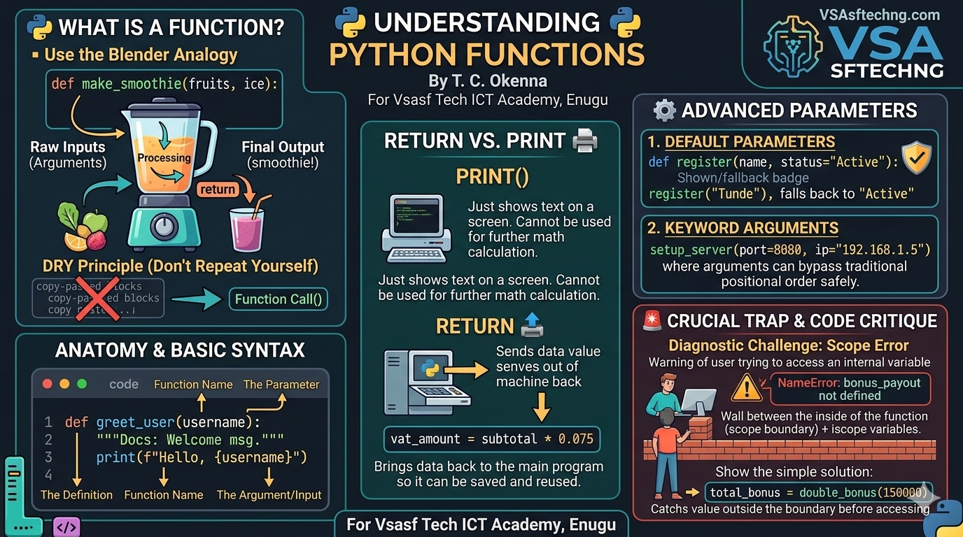
Lecture Notes: Introduction to Python Functions. By T. C. OkennaFunctions are self-contained blocks of reusable code designedto perform a specific, single action. By shifting code away from long,repetitive scripts into modular functions, developers make theirapplications significantly more organized, easier to test, and maintainable.📋 Lesson OverviewTarget Audience: Beginner to Intermediate Python LearnersDuration: 60 MinutesPrerequisites: Python variables, operational data types,and logical conditional blocks (if/else).Learning Objectives: By the end of this lesson, students will be able to:Define and call functions using the def keyword.Differentiate between parameters (inputs) and arguments (actual values).Return calculations using the return statement.Implement positional, keyword, and default parameters correctly.👩‍🏫 Lesson Structure1. Introduction: The "Why" of Functions (10 Mins)The Real-World Analogy: A kitchen blender. The blender has adefined mechanism. You pass raw inputs into it (fruits, ice),it processes them internally according to a fixed design, and it pours outa final result (a smoothie). You don't rebuild the blender everytime you want a drink; you just call upon it.The DRY Principle: Don't Repeat Yourself. If you copy-paste the samefive lines of code three or more times across a script,it should be refactored into a reusable function.2. Basic Syntax & Anatomy of a Function (15 Mins)A function definition uses the def keyword, followed by a uniquefunction name, parental parameters inside parentheses,a colon (:), and an indented block of code.python# 1. Defining the Function (Building the Blender) def greet_user(username): """Docstring: Prints a welcome message to a user.""" print(f"Welcome back to the system, {username}!") # 2. Calling the Function (Using the Blender) greet_user("Chinedu") # Output: Welcome back to the system, Chinedu! greet_user("Amaka") # Output: Welcome back to the system, Amaka! Use code with caution.Parameters vs. ArgumentsParameter: The structural variable placeholder listedinside the function definition (username).Argument: The actual, concrete value passed intothe function when invoking it ("Chinedu").3. Returning Values vs. Printing (15 Mins)A very common point of confusion for beginners isthe difference between print() and return.print() simply displays text on the screen for a humanto look at. It has no structural computation value.return terminates function execution and sends data back to themain program stream so it can be assigned to variablesor utilized in subsequent math calculations.python# Real-World Scenario: E-commerce VAT sales calculation def calculate_vat(subtotal): vat_amount = subtotal * 0.075 # 7.5% VAT rate return vat_amount # Handing the computation value back # Capturing the returned value to use later order_vat = calculate_vat(12000) final_invoice = 12000 + order_vat print(f"Total Invoice Cost: N{final_invoice}") # Output: Total Invoice Cost: N12900.0 Use code with caution.4. Advanced Parameter Handling (15 Mins)Default ParametersYou can assign default values to parameters. If an argumentis missing during execution, the default value acts as a safe fallback.python# Real-World Scenario: User profile setup with default status values def register_member(name, status="Active"): return f"Member: {name} | Account Status: {status}" print(register_member("Tunde")) # Output: Member: Tunde | Account Status: Active print(register_member("Fatima", "Suspended")) # Output: Member: Fatima | Account Status: Suspended Use code with caution.Positional vs. Keyword ArgumentsPositional: Arguments matched purely by theirspecific placement sequence order.Keyword: Arguments explicitly linked by name (parameter_name=value),allowing you to completely pass variables out of sequence order safely.pythondef setup_server(ip, port, Protocol="HTTPS"): return f"Hosting server at {ip}:{port} via {Protocol}" # Using Keyword arguments out of original definition order print(setup_server(port=8080, ip="192.168.1.5")) # Output: Hosting server at 192.168.1.5:8080 via HTTPS Use code with caution.🎯 Diagnostic Challenge & Code CritiqueAsk the Class: Look at this block of script logic. What will printwhen we execute it, what structural variable scopeerror did the developer make, and how do we resolve it?pythondef double_bonus(salary): bonus_payout = salary * 2 return bonus_payout employee_salary = 150000 double_bonus(employee_salary) print(bonus_payout) # 💥 CRASH! Use code with caution.Expected Solution CritiqueThe Error: This script throws a NameError: name 'bonus_payout' is not defined.The Reason: Variable scope rules. The variable bonus_payoutis defined inside the function. It lives and dies exclusivelywithin that internal scope ecosystem. The main program scope(global line footprint) cannot look inside the function boundary box directly.Furthermore, although the function returned the value, thedeveloper forgot to save it into an outside variable!The Refactored Fix: Catch the return data stream safely:pythonemployee_salary = 150000 # Store the returned outcome value inside #a globally visible variable frame total_bonus = double_bonus(employee_salary) print(total_bonus) # Output: 300000 Use code with caution.For Vsasf Tech ICT Academy, Enugu

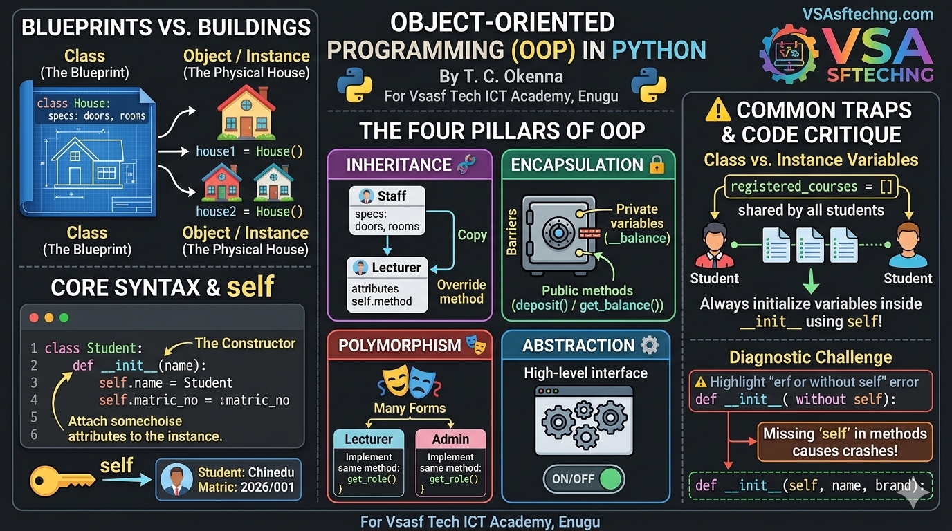
Lecture Notes: Object-Oriented Programming (OOP) in Python. By T. C. OkennaObject-Oriented Programming (OOP) is a programming paradigm thatorganizes software design around data, or objects, rather than functionsand logic. It allows developers to bundle related properties and behaviorsinto individual, reusable structures, mirroring how real-world entities exist.📋 Lesson OverviewTarget Audience: Intermediate Python LearnersDuration: 60 MinutesPrerequisites: Python functions, dictionaries, and basic loop constructs.Learning Objectives: By the end of this lesson, students will be able to:Differentiate between a Class and an Object.Implement instance attributes using the __init__ constructor method.Explain and apply the four pillars of OOP: Inheritance, Polymorphism,Encapsulation, and Abstraction.👩‍🏫 Lesson Structure1. Introduction: Blueprints vs. Buildings (10 Mins)The Real-World Analogy: Think of an architectural blueprint for a house.The blueprint itself isn't a house; it's a design document containingspecifications (number of rooms, doors) and capabilities (wiring, plumbing layouts).A Class is that architectural blueprint.An Object (or Instance) is the actual physical house built usingthat blueprint. You can build 50 completely distinct houses from one single blueprint.2. Core Syntax: Classes, Objects, and self (15 Mins)Defining a Class and ConstructorThe __init__ method is the constructor. It initializes an object'sstate when it is created. The self keyword represents thespecific instance of the class currently being modified.python# Real-World Scenario: Simulating a student registration profile class Student: # The Constructor Method def __init__(self, name, matric_no, department): self.name = name # Instance Attribute self.matric_no = matric_no # Instance Attribute self.department = department # Instance Attribute # Instance Method def display_profile(self): return f"Student: {self.name} | Matric: {self.matric_no} | Dept: {self.department}" # Instantiating (Creating) distinct objects student1 = Student("Chinedu", "2026/001", "Computer Science") student2 = Student("Amaka", "2026/042", "Electronic Engineering") print(student1.display_profile()) # Output: Student: Chinedu | Matric: 2026/001... print(student2.name) # Output: Amaka Use code with caution.3. The Pillars of OOP (25 Mins)🧬 Pillar 1: InheritanceInheritance allows a new child class to adopt the attributesand methods of an existing parent class, eliminating redundant code.python# Parent Class class Staff: def __init__(self, name, staff_id): self.name = name self.staff_id = staff_id def get_role(self): return "General Staff Member" # Child Class inheriting from Staff class Lecturer(Staff): def __init__(self, name, staff_id, course_assigned): super().__init__(name, staff_id) # Call parent constructor self.course_assigned = course_assigned # Method Overriding (Polymorphism) def get_role(self): return f"Lecturer teaching {self.course_assigned}" lecturer = Lecturer("Dr. Okoye", "L-902", "Python Programming") print(lecturer.get_role()) # Output: Lecturer teaching Python Programming Use code with caution.🔒 Pillar 2: EncapsulationEncapsulation restricts direct access to an object's componentmethods and variables to prevent accidental manipulation.In Python, we prefix variable names with a doubleunderscore (__) to denote private variables.pythonclass BankAccount: def __init__(self, owner, initial_balance): self.owner = owner self.__balance = initial_balance # Private attribute # Getter method to read private data safely def get_balance(self): return self.__balance # Setter method to update private data safely with validation def deposit(self, amount): if amount > 0: self.__balance += amount else: print("Invalid deposit amount!") account = BankAccount("Kelechi", 50000) # print(account.__balance) # 💥 CRASH! Throws AttributeError account.deposit(15000) print(account.get_balance()) # Output: 65000 Use code with caution.4. ⚠️ Common Pitfalls: Class vs. Instance Variables (5 Mins)Instance Variables: Variables defined inside constructormethods using self. They belong uniquely to that specific object.Class Variables: Variables declared directly in the class body outsideany method. They are shared collectively by all instances of that class.python# 🚫 THE INCORRECT USE-CASE (Class variable trap) class Registry: registered_courses = [] # Shared by ALL student instances accidentally! def __init__(self, student_name): self.student_name = student_name student_a = Registry("Tunde") student_b = Registry("Fatima") student_a.registered_courses.append("CSC 201") # Fatima has unexpectedly been registered for Tunde's course! print(student_b.registered_courses) # Output: ['CSC 201'] Use code with caution.🎯 Diagnostic Challenge & Code CritiqueAsk the Class: Examine this script snippet. Why will it throw a runtime crash exception when executed, and how should we refactor it?pythonclass SmartDevice: def __init__(name, brand): name = name brand = brand def power_on(): print(f"{name} is now powered online.") phone = SmartDevice("Pixel 8", "Google") phone.power_on() # 💥 CRASH! Use code with caution.Expected Solution CritiqueThe Error: This script breaks with a missing argumentexception or local scope lookup errors (NameError: name 'name' is not defined).The Reason:The developer forgot to pass self as the very firstposition parameter in both __init__ and power_on().The variables inside the constructor were assigned locally (name = name) instead of attaching them structurally tothe object scope instance using self.name = name.The Refactored Fix:pythonclass SmartDevice: def __init__(self, name, brand): # Added self self.name = name # Bound to object self.brand = brand def power_on(self): # Added self print(f"{self.name} is now powered online.") Use code with caution.For Vsasf Tech ICT Academy, Enugu

Lecture Notes: Regression Analysis with Python. By T. C. OkennaRegression Analysis is a fundamental statistical and machine learning technique used to model, investigate, and quantify the relationship between a dependent variable (target/outcome) and one or more independent variables (predictors/features).📋 Lesson OverviewTarget Audience: Intermediate Python Learners & Aspiring Data AnalystsDuration: 60 MinutesPrerequisites: Python fundamentals, core packages (Pandas, NumPy), and foundational algebra.Learning Objectives: By the end of this lesson, students will be able to:Differentiate between Simple and Multiple Linear Regression.Implement an end-to-end regression model pipeline using the Scikit-Learn Regression API.Interpret key parameters like coefficients, intercept, and evaluation metrics.👩‍🏫 Lesson Structure1. Introduction: The "Why" of Regression (10 Mins)The Real-World Analogy: Predicting your monthly electricity bill. The bill doesn't change randomly; it depends predictably on measurable factors like daily temperature, the square footage of your home, and the total runtime of your air conditioner.The Objective: We fit a line (or hyperplane) through data points so we can predict continuous numerical variables based on input inputs.The Mathematics:\(\^{y}=\beta {0}+\beta {1}X_{1}+\beta {2}X{2}+...+\beta {n}X{n}\)\(\^{y}\): The predicted value (Dependent variable).\(\beta _{0}\): The Intercept (Where the line crosses the y-axis when \(X=0\)).\(\beta_1, \beta_2\): The Coefficients (The slope/weight showing how much \(y\) updates per unit change in \(X\)).2. Core Concepts: Simple vs. Multiple Regression (10 Mins)TypeIndependent Variables (\(X\))Use-Case ExampleSimple Linear RegressionExactly One (\(X_{1}\))Predicting home value based only on its size (square feet).Multiple Linear RegressionTwo or More (\(X_1, X_2, \dots\))Predicting home value based on size, location rating, and construction year.3. Step-by-Step Implementation with Python (25 Mins)Here is a real-world coding solution predicting real estate prices based on spatial properties.pythonimport numpy as np import pandas as pd from sklearn.model_selection import train_test_split from sklearn.linear_model import LinearRegression from sklearn.metrics import mean_squared_error, r2_score # 1. Create a mock Real Estate dataset data = { 'Size_SqFt': [1500, 1800, 2400, 3000, 1200, 2100, 1600, 2800], 'Bedrooms': [3, 3, 4, 4, 2, 3, 3, 4], 'Price_USD': [250000, 290000, 380000, 470000, 190000, 330000, 265000, 430000] } df = pd.DataFrame(data) # 2. Separate Features (X) and Target (y) X = df[['Size_SqFt', 'Bedrooms']] y = df['Price_USD'] # 3. Split dataset into Training (80%) and Testing (20%) sets X_train, X_test, y_train, y_test = train_test_split(X, y, test_size=0.2, random_state=42) # 4. Instantiate and Train the Linear Regression Model model = LinearRegression() model.fit(X_train, y_train) # 5. Generate Predictions using the test partition y_pred = model.predict(X_test) # 6. Extract Parameters print(f"Intercept (Beta 0): {model.intercept_:.2f}") print(f"Coefficients (Beta 1, Beta 2): {model.coef_}") Use code with caution.4. Evaluating Model Performance (10 Mins)To measure how well our model fits the data, we use standard evaluation metrics:Mean Squared Error (MSE): Measures the average squared difference between actual values and predicted values. Lower is better.\(R^{2}\) Score (Coefficient of Determination): Represents the proportion of variance in the dependent variable that is predictable from the independent variables. Ranging from 0 to 1 (Higher is better, where 1.0 means a perfect fit).python# Continuing from the script above... mse = mean_squared_error(y_test, y_pred) r2 = r2_score(y_test, y_pred) print(f"Mean Squared Error: {mse:.2f}") print(f"R2 Score: {r2:.4f}") # e.g., 0.9850 means 98.5% variance explained Use code with caution.5. ⚠️ Crucial Traps & Checklist (5 Mins)When applying linear regression in production, look out for these pitfalls:Non-Linear Relationships: Linear regression assumes a straight-line relationship. If your data bends dramatically, consider Polynomial features or alternate models.Multicollinearity: If your independent variables (\(X_{1}\) and \(X_{2}\)) are highly correlated with each other (e.g., house size in square feet vs house size in square meters), it destabilizes coefficient tracking. Drop one of the redundant variables.🎯 Diagnostic Challenge & Code CritiqueAsk the Class: Look closely at this implementation fragment. What major data data structural mistake did the developer make before fitting the model?pythonimport pandas as pd from sklearn.linear_model import LinearRegression # Loading regional sales logs df = pd.DataFrame({ 'City': ['Enugu', 'Lagos', 'Abuja', 'Enugu'], 'Marketing_Spend': [500, 1200, 900, 600], 'Revenue': [4500, 11000, 8500, 5200] }) X = df[['City', 'Marketing_Spend']] y = df['Revenue'] model = LinearRegression() model.fit(X, y) # 💥 CRASH! Use code with caution.Expected Solution Critique:The Error: This script throws a ValueError: could not convert string to float: 'Enugu'.The Reason: Linear regression is a purely mathematical optimization algorithm. It cannot handle raw string data like categorical city names directly.The Fix: Convert the string column into numerical vectors before fitting. Use data encoding techniques like One-Hot Encoding via pd.get_dummies(df, columns=['City']) to prepare it correctly.For Vsasf Tech ICT Academy, Enugu

Lecture Notes: Lists & Dictionary Manipulation with Loops. By T. C. OkennaThis lesson covers iterating through and modifying Python data structures.Students will learn how to combine loops with lists and dictionaries to dynamicallyfilter data, aggregate values, and safely update collections in real-world applications.Lesson OverviewTarget Audience: Intermediate Python LearnersDuration: 60 MinutesPrerequisites: Python Lists, Python Dictionaries, and basic for / while loop syntax.Learning Objectives: By the end of this lesson, students will be able to:Traverse lists and nested structures using loops.Perform data aggregation (sums, counts) and filtering dynamically.Extract keys, values, and items from dictionaries during iteration.Avoid common pitfalls like mutating a collection while iterating over it.Lesson Structure1. Introduction: The Need for Automation (10 Mins)The Problem: Modifying index variables or dictionary keys manually is fine for one or two data points.But what if you need to apply a 10% discount to 10,000 items in an e-commerce catalog,or filter out spam accounts from a subscriber list of millions?The Solution: Combining loops with data structures allows your program toautomate structural data changes efficiently based on logical rules.2. List Manipulation with Loops (15 Mins)Modifying List Elements by IndexTo update items within an existing list during execution, you must use their indices.The range(len()) pattern allows you to target each element directly.python# Real-World Scenario: Processing a list of e-commerce prices to apply a 10% discount prices = [100.0, 250.0, 75.0, 500.0] for i in range(len(prices)): prices[i] = prices[i] * 0.9 # Reduce each item by 10% print(prices) # Output: [90.0, 225.0, 67.5, 450.0] Use code with caution.Filtering Data into New ListsInstead of updating the existing structure, a very common practice isevaluating elements and using the .append() method to build a filtered collection.python# Real-World Scenario: Filtering high-value transactions for fraud review transactions = [120, 4500, 80, 2300, 15, 6000] flagged_transactions = [] for amount in transactions: if amount >= 2000: flagged_transactions.append(amount) print(flagged_transactions) # Output: [4500, 2300, 6000] Use code with caution.3. Dictionary Manipulation with Loops (15 Mins)When looping through dictionaries, you can iterateover keys, values, or key-value pairs concurrently.Updating Specific Dictionary ValuesUsing .items() unzips the dictionary entries into key and valuevariables, making conditional updates clean and readable.python# Real-World Scenario: Increasing the stock count of low inventory items warehouse_stock = {"Laptops": 12, "Mice": 3, "Monitors": 5, "Keyboards": 2} for item, count in warehouse_stock.items(): if count < 5: warehouse_stock[item] += 20 # Add emergency restocking batch print(warehouse_stock) # Output: {'Laptops': 12, 'Mice': 23, 'Monitors': 5, 'Keyboards': 22} Use code with caution.Dynamic Aggregation & InversionYou can loop through structural collections to createentirely new transformed calculations or mappings.python# Real-World Scenario: Reversing a data route mapping server_routes = {"Server_A": "192.168.1.1", "Server_B": "192.168.1.2"} ip_to_server = {} for server, ip in server_routes.items(): ip_to_server[ip] = server # Swap key and value print(ip_to_server) # Output: {'192.168.1.1': 'Server_A', '192.168.1.2': 'Server_B'} Use code with caution.4. Advanced Concept: Handling Nested Collections (10 Mins)Real-world systems pass complex JSON strings that translate directlyto lists filled with nested dictionaries. Unpacking them requires acombination of nested access loops.python# Real-World Scenario: Calculating custom invoice run totals orders = [ {"customer": "Alice", "items": [50, 100, 20]}, {"customer": "Bob", "items": [200, 300]}, {"customer": "Charlie", "items":} ] for order in orders: total_spent = 0 # Loop through the list nested inside the current dictionary for price in order["items"]: total_spent += price print(f"{order['customer']} spent a total of ${total_spent}") # Output: # Alice spent a total of $170 # Bob spent a total of $500 # Charlie spent a total of $15 Use code with caution.5. Crucial Trap: Mutating While Iterating (5 Mins)The Golden Rule: Never add or remove elements directly from a dictionaryor list while looping over that specific variable layout. This causesunexpected logic skipping or throws runtime exceptions.python# BAD CODE: Will break or skip elements active_users = {"A1": True, "B2": False, "C3": False} for user_id, active in active_users.items(): if not active: del active_users[user_id] # Throws RuntimeError: dictionary changed size during iteration Use code with caution.python# GOOD CODE: Iterate over a copy of the keys/structure instead active_users = {"A1": True, "B2": False, "C3": False} for user_id in list(active_users.keys()): if not active_users[user_id]: del active_users[user_id] # Perfectly safe execution print(active_users) # Output: {'A1': True} Use code with caution.Diagnostic Challenge & Code CritiqueAsk the Class: Look closely at this loop block. What does the developer ntend to do, what error will it crash into, and how do we resolve it?pythonlogins = [10, 0, 15, 0, 22, 0, 8] # Intention: Clean up system database logs by purging zero login cycles for activity in logins: if activity == 0: logins.remove(0) print(logins) Use code with caution.Expected Solution CritiqueThe Trap: While it might not crash with an explicit exception,it creates a silent semantic bug. When .remove() alters the list, indices shift leftward.The iteration loop jumps ahead, skipping the very next structural index element.The Output Result: It prints [10, 15, 0, 22, 8]. It completely skipped one of the zeros!The Fix: Use a list comprehension to construct a clean output copy:logins = [activity for activity in logins if activity != 0]For Vsasf Tech ICT Academy, Enugu